A post by Jindřich Mynarz of the University of Economics, Prague

Let’s say there were two EU-funded projects: a Greek one from 2013 that cost 1 million eur, and a Romanian one from 2007 that cost 4 million lei. Which of the projects was more expensive? While this question seems deceptively simple, providing a correct answer is not as straightforward as we might expect. Moreover, the ability to compare money is essential for analyses of fiscal data, so it is important we get this answer right.

When comparing money across time and space we need to take into account the context in which the money was spent. This context is primarily set by a country and a year. The country determines the currency of the monetary amount and combined with year it determines the price levels, which account for inflation. As the European System of Accounts 2010 says: “The fact that countries have different price levels and currencies poses a challenge to interspatial comparisons of prices and volumes” (p. 303). However, with the contextual data provided, we can attempt cross-country comparisons over time.

In order to arrive at a correct answer to our question above, we need to compare the amounts of money not as absolute numbers but in terms of their value. Instead of comparing their nominal values, we need to compare their real values; typically corresponding to purchasing powers.

Normalization method

There is a simple statistical method that can help us approximate the real values of monetary amounts. This method uses exchange rates to convert the amounts to a single currency and then applies GDP deflators, which adjust the amounts for different price levels in different countries and times. GDP deflator is a price index based on gross domestic product (GDP) of a country that measures changes in price levels with respect to a specific base year. Alternative normalization methods, including the use of consumer price indices, can be found in Statistical literacy guide: How to adjust for inflation by Gavin Thompson.

We can start with a naïve comparison that ignores currencies, using which 4 million seems obviously more than 1 million. Even though this conclusion is clearly ill-judged, it is often the farthest we can get when the currencies are unknown or not specified explicitly in the analysed datasets. We can improve our answer to the question if we know the currencies of the compared amounts and their relative exchange rate. Given that in 2013 an euro was worth 4.419 lei we can calculate that 4 million lei corresponds to 0.9 million euro and conclude that, contrary to our initial naïve guess, the Romanian project was cheaper than the Greek one. Nevertheless, currency conversion does not suffice, because exchange rates do not reflect the relative purchasing powers of the currencies in their markets over time. This is why we need the GDP deflator. With the deflator nominal amounts can be normalized to real amounts using the following formula.

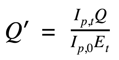
Normalization of monetary amounts using exchange rates and GDP deflators

In this formula Q is an amount of money, I_p,t is the price index for the target year to which we normalize, I_p,0 is the price index for the original year when Q was spent, E_t is the exchange rate to euro for the target year, and Q’ is the normalized amount of money. The target year is chosen as the most recent year in the normalized data. In our example we have data from 2007 and 2013, so we pick 2013 as our target year. Base year for the GDP deflator is chosen as the target year or as its nearest preceding year for which we have GDP deflators. We use the GDP deflators in euro for the EU member states published by the Eurostat, which are available with base in every 5^th year (e.g., 2005, 2010 etc.), and so we use 2010 as our base year. Applying this calculation on the example amounts reveals that the Romanian project was in fact worth approximately 1.3 million euro, making it in turn 31.6 % more expensive than the Greek project. Due to the rapid inflation of the Romanian leu between 2007 and 2013 the currency was significantly devalued, thus accounting for the difference of the real values of the compared projects.

While we can get a correct answer using this calculation, gathering the inputs needed by this method can be tedious. Fortunately, we can automate this process using linked open data.

Using linked open data

The question we started this post with can be answered by combining different kinds of data. In order to solve our question, we need to combine our data on EU projects with two datasets: data on exchange rates and data containing GDP deflators. Solving problems by combining different kinds of data is what linked data excels at.

We can combine our dataset on EU projects with two datasets published by Eurostat: the yearly averages of exchange rates of national currencies to euro and the dataset on GDP. While the original data is provided as tab-separated values (TSV), Linked Statistics provides the data as linked data in RDF described by the Data Cube Vocabulary, which makes it easier to combine it with other data. The chosen datasets can be joined via country (and in turn by the country’s currency) and year. Following the linked data principles, the entities by which we join the datasets must either reuse the same identifiers (IRIs) or use IRIs that are linked as being equivalent.

We can implement the described method in SPARQL, which is a query language for RDF. In order to simplify the demonstration of this implementation, we provide the data on our EU-funded projects directly in the SPARQL query, as well as the target year and the deflator’s unit, both of which can be chosen automatically. GDP deflators are expected to be available in the named graph <http://eurostat.linked-statistics.org/data/nama_10_gdp> and the exchange rates should be available in the named graph <http://eurostat.linked-statistics.org/data/tec00033>. Both these datasets can be downloaded here.

In the OpenBudgets.eu project we developed a reusable pipeline fragment for LinkedPipes ETL that implements the described normalization for the datasets represented using the OpenBudgets.eu data model. This pipeline is described in the deliverable 2.2 on data optimisation, enrichment, and preparation for analysis. It can be readily reused for normalization of fiscal data from the European Union.

Conclusions

In this post we have shown how to make amounts of money better comparable by using contextual data. While we improved on our initial naïve comparison of EU projects’ costs by using a method for normalizing monetary amounts via exchange rates and GDP deflators, we have taken for granted that the projects were comparable. We made this unwarranted assumption for the sake of demonstration of the described method. In fact, oblivious to the nature of the compared projects, we may have been comparing apples to oranges. The presented method is thus only the first step towards the goal of making monetary amounts in fiscal data comparable and most of the challenges of comparative analyses remain to be solved.